Phone Vision 18 – Erosion and Dilation

23 03 2011

Our exploration of set theory last time was a precursor to discussing dilation and erosion.  Simply put, dilation makes things bigger and erosion makes things smaller.  Seems obvious right?  Let’s see if the mathematicians can muck it up.

Translation

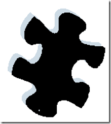
This is not necessarily a fundamental set operation, but it is critical for what we will be doing. Translation can be described as shifting the pixels in the image. We can move it in both the x and y directions and we will represent the amount of movement using a point. To translate the set then, we simply add that point to every element of the set. For instance, using the point (20, 20) the puzzle is moved down 20 pixels and right 20 pixels like this:

image

The light blue area marks the original location.

Dilation

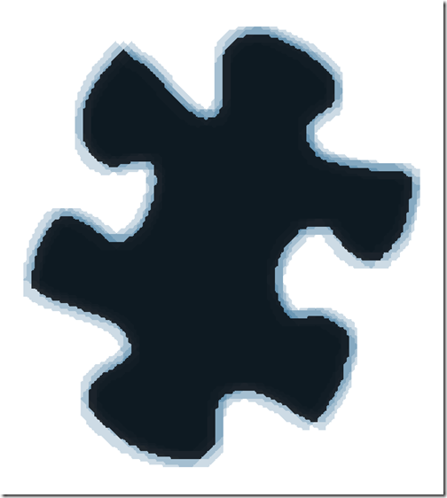
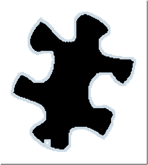
Dilation is an extension of translation from a point to a set of points. If you union the sets created by each translation you end up with dilation.  In the following diagram, the black pixels represent the original puzzle piece.  The light blue halo represents several translations of the original.  Each translation is translucent so I have tried to make the image large enough so you can see the overlap.  Notice how the hole is missing?

image

The set of points that were used to create the translated sets is called the structuring element.  A common structuring element is

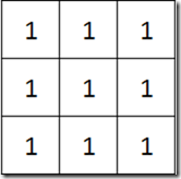
{ (-1,-1), (0,-1), (1,-1),(-1,0), (0,0), (1,0),(-1,1), (0,1), (1,1) }

This will expand the image by one pixel in every direction.  If we think about this as a binary image, it might be represented by this:

image

Kinda reminds me of one of our convolution kernels.  Structuring elements are often called “probes”.  This one is centered at (0,0).

Using the PixelSet we created last time, the code is pretty straightforward.

public void Dilate(PixelSet structuringElem)

{

    PixelSet dilatedSet = new PixelSet();

    foreach(int translateY in structuringElem._pixels.Keys)

    {

        foreach(int translateX in structuringElem._pixels[translateY])

        {

            PixelSet translatedSet = new PixelSet();

            foreach (int y in _pixels.Keys)

            {

                foreach(int x in _pixels[y])

                {

                    translatedSet.Add(x + translateX, y + translateY);

                }

            }

            dilatedSet.Union(translatedSet);

        }

    }

    _pixels = new Dictionary<int,List<int>>(dilatedSet._pixels);

}

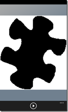
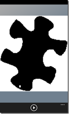
Here is the puzzle piece dilated by one pixel in all directions.  The hole is gone.

image

Erosion

Erosion is similar to dilation except that our translation is subtraction instead of addition and we are finding the intersection instead of the union.  Here is an image that has been eroded by 10 pixels in all directions.  The light blue area is the original puzzle.


image


public void Erode(PixelSet structuringElem)

{

    PixelSet erodedSet = new PixelSet(this);

    foreach (int translateY in structuringElem._pixels.Keys)

    {

        foreach (int translateX in structuringElem._pixels[translateY])

        {

            PixelSet translatedSet = new PixelSet();

            foreach (int y in _pixels.Keys)

            {

                foreach (int x in _pixels[y])

                {

                    translatedSet.Add(x – translateX, y – translateY);

                }

            }

            erodedSet.Intersect(translatedSet);

        }

    }

    _pixels = new Dictionary<int,List<int>>(erodedSet._pixels);

}


Here is the puzzle eroded by one pixel in all directions.  That hole is a little bigger.

image

Summary

Like I said at the beginning, dilation makes things bigger and erosion makes things smaller.  Interestingly, erosion is simply the dilation of the background and dilation is the erosion of the background.

Download Code

http://cid-88e82fb27d609ced.office.live.com/embedicon.aspx/Blog%20Files/PhoneVision/PhoneVision%2018%20-%20Erosion%20and%20Dilation.zip

Up Next: Opening and Closing


Phone Vision 17–Sets

16 03 2011

Last time we were able to get a pretty decent binary image.  The question is, what do we do with it?  Before we can answer that, we need to make sure you’ve got a basic understanding of set theory.

Sets

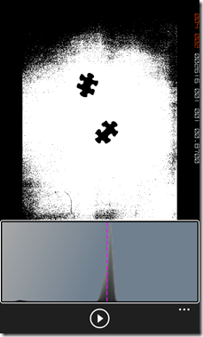
In a binary image we can think of the objects of interest as a set of points.  Here is our binary image from last time:

image

I am going to focus on just the top puzzle piece so let’s extract it.  (The code for extracting this is not important for this lesson, but it is included in the code as GetPuzzleImage).

image

We are going to be working with this image for a while.  In this case, the black pixels will represent members of our set.

Universe

The universe is the set of all possibilities.  In the case of image processing this is typically the set of all of the pixels.  I have seen this referred to as E2 (for 2-dimensional Euclidean space).  In our case, the universe is…

image

As expected, the set of every possibility is all black.  This is important some operations rely on this set.

Empty Set

The empty set is, well, empty.

image

Since the boundary for our image is not a specified size, this is just an empty image. If the universe was a specified size then the empty set would often be represented by a completely white image.

Complement

The complement is everything in the universe that is not in the set.  The complement of our puzzle piece:

image

The puzzle piece is now a hole in the black image.

Union (⋃)

The union is the set of all elements in either of two sets.  If you have been playing along, this is very similar to the | (binary OR) operation mentioned in lesson three. Below we union the puzzle set with the set of its complement.  The output is the universe.

image

image

image

Intersection (⋂)

Finally, the intersection is the set of all shared members of two sets.  Below we intersect the puzzle set with its complement.  This is similar to the & (binary AND) operations mentioned way back in lesson 2.  Since the complement of a set  doesn’t share any elements with the original set the output is going to be the empty set.

imageimageimage

Pixel Set

In order to demonstrate these concepts (and a few in the future) I created a class called PixelSet that behaves similar to a mathematical set. 

Caution: This set is not optimized for use in actual applications.  You’ve been warned.

Elements

The elements of the set are represented by a Dictionary.

Dictionary<int, List<int>> _pixels = new Dictionary<int, List<int>>();

The key is the y-value for the pixel and the List<int> represents all x-values in that row.


Add


public void Add(int x, int y)

{

    List<int> columns = new List<int>();

    if (!_pixels.ContainsKey(y))

    {

        _pixels.Add(y, columns);

    }

    else

    {

        columns = _pixels[y];

    }


    if (!columns.Contains(x))

    {

        columns.Add(x);

    }

}


The add function is a little tricky because if the row (y-value) doesn’t have a representative in the set yet then we need to create a new list to contain them. If it does, then we need to use the existing list.


Remove


public void Remove(int x, int y)

{

    if (_pixels.ContainsKey(y))

    {

        if (_pixels[y].Contains(x))

        {

            _pixels[y].Remove(x);

            if (_pixels[y].Count == 0)

            {

                _pixels.Remove(y);

            }

        }

    }

}


Remove is included for completeness, but I’m not calling it from any location in the code.


Union


public void Union(PixelSet otherSet)

{

    foreach (int key in otherSet._pixels.Keys)

    {

        foreach (int col in otherSet._pixels[key])

        {

            Add(col, key);

        }

    }

}


A possible optimization here is to loop through the smallest set.  You would need to maintain a count, but since new members are added through Add that should be easy.


Intersect


public void Intersect(PixelSet otherSet)

{

    PixelSet intersection = new PixelSet();

    foreach (int key in otherSet._pixels.Keys)

    {

        if (_pixels.ContainsKey(key))

        {

            foreach (int col in otherSet._pixels[key])

            {

                if (_pixels[key].Contains(col))

                {

                    intersection.Add(col, key);

                }

            }

        }

    }

    _pixels = new Dictionary<int, List<int>>(intersection._pixels);

}


Once again you could change this to loop through the smallest set to speed this up.


Summary
 

I expect this will have been a review for many readers, but it’s important to have a grasp of this information before we head into the next lesson regarding erosion and dilation.  I’d also like to reiterate that this is not optimized for image processing.  My HD7 takes almost 8 times longer to execute some of these tight loops.


Download Code

http://cid-88e82fb27d609ced.office.live.com/embedicon.aspx/Blog%20Files/PhoneVision/PhoneVision%2017%20-%20Set%20Operations.zip

Up Next: Erosion and Dilation


Phone Vision 16 – Binary Images

9 03 2011

When we are creating a binary image we are defining objects of interest.  Defining these objects is very specific to the task at hand.  In some cases a simple threshold will work while others require a more complex approach such as color segmentation, edge detection, or something even more sinister.

Thresholding

The most common way to create a binary image from a grayscale image is to pick an intensity threshold (also known as gray-level segmentation).  Everything below the threshold becomes a pixel of interest (black).  Everything else is not (white).  Let’s explore a few methods for picking that threshold.

The Image

Interestingly, this picture is a white piece of poster board (not blue) with some dark puzzle pieces on it.  If you look closely you can see the famous HD7 pink tint.  The image on the right is simply converted to grayscale using the average of the RGB values.

imageimage

Mean Threshold

Almost every time an image processing problem arises and a simple average is a possible answer my gut tells me to go for it.  In this case, my gut is going to lead me astray, but first some code:

WriteableBitmap ToAverageBinary(WriteableBitmap grayscale)

{

    WriteableBitmap binary =

        new WriteableBitmap(grayscale.PixelWidth,

            grayscale.PixelHeight);


    int[] histogramData = new int[256];

    int maxCount = 0;


    //first we will determine the histogram

    //for the grayscale image

    for (int pixelIndex = 0;

        pixelIndex < grayscale.Pixels.Length;

        pixelIndex++)

    {

        byte intensity = (byte)grayscale.Pixels[pixelIndex];


        //simply add another to the count

        //for that intensity

        histogramData[intensity]++;


        if (histogramData[intensity] > maxCount)

        {

            maxCount = histogramData[intensity];

        }

    }


    //now we need to figure out the average intensity

    long average = 0;

    for (int intensity = 0; intensity < 256; intensity++)

    {

        average += intensity * histogramData[intensity];

    }


    //this is our threshold

    average /= grayscale.Pixels.Length;


    for (int pixelIndex = 0;

        pixelIndex < grayscale.Pixels.Length;

        pixelIndex++)

    {

        byte intensity = (byte)grayscale.Pixels[pixelIndex];


        //now we’re going to set the pixels

        //greater than or equal to the average

        //to white and everything else to black

        if (intensity >= average)

        {

            intensity = 255;

            unchecked { binary.Pixels[pixelIndex] = (int)0xFFFFFFFF; }

        }

        else

        {

            intensity = 0;

            unchecked { binary.Pixels[pixelIndex] = (int)0xFF000000; }

        }

    }


    //note that this is the ORIGINAL histogram

    //not the histogram for the binary image

    PlotHistogram(histogramData, maxCount);


    //this is a line to show where the

    //average is relative to the rest of

    //the histogram

    Line averageLine = new Line();

    averageLine.X1 = HistogramPlot.Width * average / 255;

    averageLine.X2 = HistogramPlot.Width * average / 255;

    averageLine.Y1 = 0;

    averageLine.Y2 = HistogramPlot.Height;

    averageLine.Stroke = new SolidColorBrush(Colors.Magenta);

    averageLine.StrokeThickness = 2;

    averageLine.StrokeDashArray = new DoubleCollection() { 5, 2.5 };

    HistogramPlot.Children.Add(averageLine);

    return binary;

}

image


While the puzzle pieces came through loud and clear so did a lot of garbage.  Notice how the average line (magenta) splits the peak?  This is going to lead to a large number of false black pixels.  What we want is an automated technique for shifting the threshold left.


Two Peak


If you look at the original grayscale image you’ll notice that the puzzle pieces seem to be close to the same intensity while the background is another. This is represented in the histogram by the large peak (the background) and an almost imperceptible peak toward the dark end of the spectrum (the puzzle pieces).


Finding the large peak is trivial.  It’s just the highest occurring intensity.  The small peak on the other hand is a little trickier.  It’s not the second most frequent intensity – that’s right next to the largest peak.  A little trick is to give a higher weight to intensities that are far from the highest peak.  To do this we multiply the intensity count at each point by the square of its distance to the peak.  That’s a mouthful, but it’s pretty easy.  Here’s the code:


int secondPeak = 0;

long secondPeakCount = 0;

for (int intensity = 0; intensity < 256; intensity++)

{

    long adjustedPeakCount =

        (long)(histogramData[intensity]*Math.Pow(intensity-maxPeak, 2));

    if (adjustedPeakCount > secondPeakCount)

    {

        secondPeak = intensity;

        secondPeakCount = adjustedPeakCount;

    }

}

So we calculate an adjusted count for each intensity.  By multiplying it by the square of the distance we give higher counts to those further from the first peak.  Amazingly, this works even in this case where the second peak is so small.

image

Wow!  Those results are so much better.  Notice I marked the two peaks with green and the new threshold is in magenta.

Summary

Don’t use the mean.  You might get lucky in a few cases, but in general you’ll end up in a messy situation.  That said, the two-peak solution will work well in cases where your objects are of a consistent color and that color is separate from the background.  I created this photo because I knew it would have good results.  I highly recommend you try these techniques out on your own photos so you can get a feel for when they will work and when they won’t.

We will most likely revisit different thresholding techniques for different situations when they arise, but for now we have a binary image so we’re going to see what we can do with it.

Download Code

http://cid-88e82fb27d609ced.office.live.com/embedicon.aspx/Blog%20Files/PhoneVision/PhoneVision%2016%20-%20Binary%20Images.zip

Up Next: Sets


Phone Vision 15 – Median Filters

1 03 2011

Filters, filters, filters… Tired of them yet?  Me too.  After this we’ll leave them alone for a while.  I promise.  Until then, we have work to do.

What is a median filter?  If you understand the average filter (or mean filter) then the median filter should give you no troubles at all – assuming you know what the median is.  We’ll start there.

What is the Median?

The median is the middle number of a sample.  To find it, you sort your list and pick the middle item.  Yes, it really is that simple.

Here is a random set of 9 numbers:

image

Sort them:

image

Pick the middle value:

image

Like I said, it’s simple.

Why use median instead of mean?

The median is particularly effective against certain types of noise – specifically “salt and pepper” noise (black and white specks).  Let’s assume this is the neighborhood we’re dealing with:

image

Performing the mean gives:

image

image

While the median returns:

image

image

If we expect that the 0 values are noise then the median is probably a much closer estimate.

Code

private WriteableBitmap MedianFilter(WriteableBitmap grayscale, int radius)

{

    // we are still going to create a new image

    // because we don’t want to modify the

    // old image as we are processing it

    WriteableBitmap filtered =

        new WriteableBitmap(

            grayscale.PixelWidth,

            grayscale.PixelHeight);


    // boiler plate code for our

    // histogram stuff

    int[] histogram = new int[256];

    int maxIntensity = 0;


    // the math is still easier if we create two loops

    // instead of one

    for (int y = 0; y < grayscale.PixelHeight; y++)

    {

        for (int x = 0; x < grayscale.PixelWidth; x++)

        {

            //here’s the pixel we’re centered on

            int pixel = x + y * grayscale.PixelWidth;

            byte intensity = (byte)grayscale.Pixels[pixel];


            // if we are on an edge we are going to leave it

            // as the original intensity.  you will see the

            // edges increasingly unsmoothed as the window

            // size increases.  here we are using the radius

            // to determine our bounds

            if (y <= radius – 1 ||

                x <= radius – 1 ||

                y >= grayscale.PixelHeight – radius ||

                x >= grayscale.PixelWidth – radius)

            {


                histogram[intensity]++;

                if (histogram[intensity] > maxIntensity)

                {

                    maxIntensity = histogram[intensity];

                }

                continue;

            }


            /////////////////////////////////////////////////////////

            // IMPORTANT PART ///////////////////////////////////////

            /////////////////////////////////////////////////////////

            // this list is the key

            // it contains all of the neighboring pixels

            List<byte> localIntensities = new List<byte>();

            for (int yoffset = -radius; yoffset <= radius; yoffset++)

            {

                for (int xoffset = -radius;

                    xoffset <= radius;

                    xoffset++)

                {

                    localIntensities.Add((

                        (byte)grayscale.Pixels[(x + xoffset)

                        + (y + yoffset) * grayscale.PixelWidth]));

                }

            }

            //sort the intensities

            localIntensities.Sort();

            //pick the middle value

            int medianLocalIntensity =

             localIntensities[(int)(localIntensities.Count/2.0+.5)];

            /////////////////////////////////////////////////////////

            // END IMPORTANT PART ///////////////////////////////////

            /////////////////////////////////////////////////////////


            // and now just set the color

            filtered.Pixels[pixel] = (255 << 24)

                | (byte)medianLocalIntensity << 16

                | (byte)medianLocalIntensity << 8

                | (byte)medianLocalIntensity;


            histogram[(byte)medianLocalIntensity]++;

            if (histogram[(byte)medianLocalIntensity] > maxIntensity)

            {

                maxIntensity = histogram[(byte)medianLocalIntensity];

            }

        }

    }


    PlotHistogram(histogram, maxIntensity);

    return filtered;

}


Results

Taking a simple gray image I added salt and pepper noise to the image then performed a median filter and an average filter to it.  The results are stunning.

imageimage

                flat gray image                              10% salt and pepper noise

imageimage

           after median filtering                      after mean filtering

There are a few specks after applying the median filter, but the noise is removed pretty well.  The average filter performed dismally to say the list.

Summary

If you expect salt and pepper noise then the median filter is great tool to have in your toolbox.  If you want you can explore max, min, and mode filters.  I don’t think we’ll cover them here unless we have a specific application for it.

Download Code

http://cid-88e82fb27d609ced.office.live.com/embedicon.aspx/Blog%20Files/PhoneVision/PhoneVision%2015%20-%20Median%20Filter.zip

(code includes salt and pepper noise generation)

Up Next: Binary Images

Feel free to leave a comment or follow @azzlsoft on Twitter if you have any questions.


Phone Vision 14 – Sobel Operators

25 02 2011

Last time we explored how we can use the rate of change between adjacent pixels to enhance a boundary between two features in an image.  Today we are going to take that one step further and isolate edges using the Sobel operators.  Hold on tight…

The Sobel Operators

A search for the Sobel operators will quickly turn up these two filters:

image

image


I created a rather colorful graphic to demonstrate some of the concepts.

image


imageimageimage

What do you notice?  Here’s what I notice:

  • All of the non-edges turn black. 
  • Diagonal edges show up in both filters. 
  • The first filter misses horizontal edges
  • The second filter misses vertical edges.

The union of these two images will give you a more complete view of the edges in the system.  If that’s all you wanted to know then you’re done and you can stop here.

I’m curious how they work so I’m going to dig deeper.

Gradient

When you are driving down a mountain you might see a sign (like the one to the right) indicating a steep grade.  The grade in the context of a mathematical function is no different.  We are trying to find the slope of the function at a given point.  This is called the gradient.

Last time we looked at how fast a function was changing by subtracting adjacent intensities.    If you think about it, it’s easy to imagine areas with a lot of change having a steep slope, right?  So have we already found the gradient?  Yes and no.  Hold on, this is going to get rough.

Subtracting the adjacent intensities, we determined the slope from one pixel to the next, but we didn’t determine the slope at the pixel.  Because we are dealing with discrete values (i.e. there is no ‘in-between’ pixels) the best we can hope for is an approximation of the slope at a pixel.  I am hoping that an example will clear this up a bit. 

Imagine the sin function represents some hilly terrain you are driving over.

image

It should be fairly apparent that at the top of the hill our grade is flat (slope = 0).  Let’s imagine we have a GPS recording our position every so often so we get an approximation of the terrain.

image

Using the same technique as the last lesson, let’s try to approximate the slope at the top of the hill.  Last time we said the change was f(x+1) – f(x).

image

Well, that’s not very good.  It turns out that if we adjust our formula ever so slightly we get much better results.  What if we use the position right before we got to the top of the hill instead of the position at the top?

image

That is a much better approximation,but what now?

Gradient Edge Detection

Let’s convert our new difference function to our filter representation. 

Remember,

  • f(x+1) = next position (right after the top)
  • f(x) = current position (at the top)
  • f(x-1) = previous position (right before the top)

so our gradient function looks like:

-1*f(x-1) + 0* f(x) + 1*f(x+1)

or

image

Following the same process in the y direction we end up with

-1*f(y-1) + 0* f(y) +1*f(y+1)

or

image

If we apply these we end up with:

imageimageimage

It’s a much weaker signal, but I can still spot the edges. 

If these filters make sense to you then you should be able to answer the following questions:

  • Why are the horizontal lines still missing in the first image?
  • And the vertical lines still missing in the second image? 
  • Why do the diagonals show up?

Separable Filters

You might be thinking, “um, I guess this is nice, but what does it have to do with the Sobel?”  Everything.

We don’t have the tools yet to completely analyze this, but the Sobel operator is a separable filter.  This means that it is a combination of two 1D filters.  Sobel is a smooth filter multiplied with the gradient filter we just built.

A couple of notes:

  • [1,2,1] is a 1D weighted smoothing filter
  • This is matrix multiplication.  If you need a refresher, check out the Kahn Academy video on the subject.  I love that place.


image

and

image

Whoa!  Mind blown.

Summary

We are starting to add some useful tools to our toolbox, but we are dancing around some really complex concepts.  Over the next few lessons we will continue working with a few more simple blur, sharpen, and edge detection routines before we jump head first into frequency analysis.

Download Code

http://cid-88e82fb27d609ced.office.live.com/embedicon.aspx/Blog%20Files/PhoneVision/PhoneVision%2014%20-%20Sobel%20Operator.zip

Up Next: Median Filter

Feel free to leave a comment or follow @azzlsoft on Twitter if you have any questions.


Phone Vision – 13 Sharpening Filters

21 02 2011

Smoothing an image was pretty intuitive.  When we are smoothing an image we are actually trying to suppress details in the image.  When we sharpen an image we are trying to do the opposite.  So, how do we do that?

Rates of Change

When we are sharpening an image we are trying to enhance the differences.  What are the differences?  Well, let’s take a look at a 1D strip of intensities:

image

If we take a cursory look at these pixels we’ll see that the intensities gradually decrease from left to right before jumping back up dramatically then dropping back down.  The dramatic ‘jumps’ are what will ultimately be enhanced when we sharpen the image.  Here they are highlighted.

image

We want to know how fast the intensities are changing.  If ∆ represents the rate of change between adjacent pixels then our rate of change looks like:

image

We just subtract the value of the next pixel from the value of the current pixel.  A little more formally, this looks like

∆(x) = f(x+1) – f(x)

Under normal conditions, some natural variation will occur pixel by pixel.  We want to ignore that natural variation and only concern ourselves when the change is drastic.  For that we will have to perform the subtraction one more time.

image

Now we can see how fast each intensity is changing.  Once again, let’s formalize this.

2(x) =∆(x+1) – ∆(x)

2(x) = (f(x+1) – f(x)) – (f(x) – f(x-1)

2(x) = f(x-1) – 2 * f(x) + f(x+1)

Implementing the 1D Case

Then the filter for our 1D case  looks like

image

If we apply this to our image we end up with this from above:

image

If we subtract this from our original image something magical happens:

image

We have sharpened the image!

In order to achieve that result, we subtracted ∆2  from the original image f.  Our new formula looks like:

sharp = f – ∆2

so in the x direction,

sharp(x) = f(x) – ∆2(x)

sharp(x) = f(x) – (f(x-1) – 2 * f(x) + f(x+1))

sharp(x) = f(x) + -f(x-1) + 2 * f(x) – f(x+1)

sharp(x) = –f(x-1) + 3*f(x) – f(x+1)

Hence, our final 1D filter:

image

Expanding to 2D

If all images were just a single strip of pixels we’d be done.  Unfortunately they aren’t, but accounting this is a pretty simple adjustment.  The first thing to notice is that the 1D case works in any direction.  If we wanted to apply the filter vertically instead of horizontally it would look like this:

image

So, how do we expand this to two dimensions?  It’s pretty easy, actually:

image

Now you have a sharpening filter that will work in two dimensions.  If you want to include the diagonals, there is no reason you can’t.  Using the exact same method the final sharpening filter becomes:

image

And we’re done!

Summary

With some luck, you will have a solid grasp of how the sharpening filter works.  If you are interested in researching this topic more, we walked through creating the Laplacian operator.  If you are comfortable with calculus, the difference functions we discussed were actually just the first derivative (∆) and the second derivative (∆2).

Having discussed the filter code at length, the code is not posted here.  The code from previous lessons will work fantastically.

Up Next: Sobel Operators


Phone Vision 12–Smoothing Filters

15 02 2011

What does it mean to smooth an image?  When I imagine a smooth surface it doesn’t have a lot of bumps or pits.  If we were to try to smooth out a rough piece of wood we would probably sand down the peaks and fill in holes.  If you apply that analogy to an image it sounds a lot like averaging a neighborhood.

Average Filter

If you remember from last time we described a neighborhood filter using a number of weights as follows:

image

A simple average would allow all of the pixels in the neighborhood to contribute equally to the average.  In that case would represent the filter as:

image

Using our code from last time, the filter looks like

int[,] filter = new int[,]

{

    { 1, 1, 1 },

    { 1, 1, 1 },

    { 1, 1, 1 }

};

And here are the results when we run it:

image

image

The original is on the left and the smoothed version is on the right.  Notice how the large objects are relatively unchanged, but the small objects have lost a lot of information.  In addition to removing noise, if we are trying to segment large objects, we can use smoothing to blur out the small objects.

Modified Filter Code

If we run this filter enough times we will eventually get every pixel to be some sort of gray.  It would be more efficient just to increase the size of the window.  Let’s modify the filtering code to accept a square filter of arbitrary size.

private WriteableBitmap Filter(WriteableBitmap grayscale, int[,] filter)

{

    // we are still going to create a new image

    // because we don’t want to modify the

    // old image as we are processing it

    WriteableBitmap filtered =

        new WriteableBitmap(

            grayscale.PixelWidth,

            grayscale.PixelHeight);


    // boiler plate code for our

    // histogram stuff

    int[] histogram = new int[256];

    int maxIntensity = 0;


    //here’s where the magic starts

    //assume the filter is square

    int length = (int)Math.Sqrt(filter.Length);

    int filterMagnitude = 0;

    for (int x = 0; x < length; x++)

    {

        for (int y = 0; y < length; y++)

        {

            filterMagnitude += filter[x, y];

        }

    }


    // this will be used for our loops

    // it’s important that our size is odd

    // so that our current pixel can be the

    // center point.

    int radius = length / 2;


    // the math is still easier if we create two loops

    // instead of one

    for (int y = 0; y < grayscale.PixelHeight; y++)

    {

        for (int x = 0; x < grayscale.PixelWidth; x++)

        {

            //here’s the pixel we’re centered on

            int pixel = x + y * grayscale.PixelWidth;

            byte intensity = (byte)grayscale.Pixels[pixel];


            // if we are on an edge we are going to leave it

            // as the original intensity.  you will see the

            // edges increasingly unsmoothed as the window

            // size increases.  here we are using the radius

            // to determine our bounds

            if (y <= radius – 1 ||

                x <= radius – 1 ||

                y >= grayscale.PixelHeight – radius ||

                x >= grayscale.PixelWidth – radius)

            {

                //maintain the original / non-smoothed

                filtered.Pixels[pixel] = (255 << 24)

                    | (byte)intensity << 16

                    | (byte)intensity << 8

                    | (byte)intensity;


                histogram[intensity]++;

                if (histogram[intensity] > maxIntensity)

                {

                    maxIntensity = histogram[intensity];

                }

                continue;

            }


            int newIntensity = 0;

            //going from -radius to radius makes the

     //math easier here too

            for (int yoffset = -radius; yoffset <= radius; yoffset++)

            {

                for (int xoffset = -radius;

                    xoffset <= radius;

                    xoffset++)

                {

                    // we loop through each pixel in the neighborhood

                    // and apply the filter. by ‘apply the filter’

                    // I mean multiply it by the appropriate weight

                    newIntensity +=

                        ((byte)grayscale.Pixels

                            [(x + xoffset)

                            + (y + yoffset) * grayscale.PixelWidth])

                        * filter[(yoffset + radius),

                        (xoffset + radius)];

                }

            }


            // scale the new intensity back

            newIntensity /= filterMagnitude;

            newIntensity =

                Math.Max(Math.Min(newIntensity, 255), 0);


            // and now just set the color

            filtered.Pixels[pixel] = (255 << 24)

                | (byte)newIntensity << 16

                | (byte)newIntensity << 8

                | (byte)newIntensity;


            histogram[(byte)newIntensity]++;

            if (histogram[(byte)newIntensity] > maxIntensity)

            {

                maxIntensity = histogram[(byte)newIntensity];

            }

        }

    }


    PlotHistogram(histogram, maxIntensity);

    return filtered;

}


Now we can really smooth the image.

A Large Filter

A 21×21 filter is about as large as I can do without having the mask wrap to the next line.

int[,] filter = new int[,]

{

    { 1, 1, 1, 1, 1, 1, 1, 1, 1, 1, 1, 1, 1, 1, 1, 1, 1, 1, 1, 1, 1 },

    { 1, 1, 1, 1, 1, 1, 1, 1, 1, 1, 1, 1, 1, 1, 1, 1, 1, 1, 1, 1, 1 },

    { 1, 1, 1, 1, 1, 1, 1, 1, 1, 1, 1, 1, 1, 1, 1, 1, 1, 1, 1, 1, 1 },

    { 1, 1, 1, 1, 1, 1, 1, 1, 1, 1, 1, 1, 1, 1, 1, 1, 1, 1, 1, 1, 1 },

    { 1, 1, 1, 1, 1, 1, 1, 1, 1, 1, 1, 1, 1, 1, 1, 1, 1, 1, 1, 1, 1 },

    { 1, 1, 1, 1, 1, 1, 1, 1, 1, 1, 1, 1, 1, 1, 1, 1, 1, 1, 1, 1, 1 },

    { 1, 1, 1, 1, 1, 1, 1, 1, 1, 1, 1, 1, 1, 1, 1, 1, 1, 1, 1, 1, 1 },

    { 1, 1, 1, 1, 1, 1, 1, 1, 1, 1, 1, 1, 1, 1, 1, 1, 1, 1, 1, 1, 1 },

    { 1, 1, 1, 1, 1, 1, 1, 1, 1, 1, 1, 1, 1, 1, 1, 1, 1, 1, 1, 1, 1 },

    { 1, 1, 1, 1, 1, 1, 1, 1, 1, 1, 1, 1, 1, 1, 1, 1, 1, 1, 1, 1, 1 },

    { 1, 1, 1, 1, 1, 1, 1, 1, 1, 1, 1, 1, 1, 1, 1, 1, 1, 1, 1, 1, 1 },

    { 1, 1, 1, 1, 1, 1, 1, 1, 1, 1, 1, 1, 1, 1, 1, 1, 1, 1, 1, 1, 1 },

    { 1, 1, 1, 1, 1, 1, 1, 1, 1, 1, 1, 1, 1, 1, 1, 1, 1, 1, 1, 1, 1 },

    { 1, 1, 1, 1, 1, 1, 1, 1, 1, 1, 1, 1, 1, 1, 1, 1, 1, 1, 1, 1, 1 },

    { 1, 1, 1, 1, 1, 1, 1, 1, 1, 1, 1, 1, 1, 1, 1, 1, 1, 1, 1, 1, 1 },

    { 1, 1, 1, 1, 1, 1, 1, 1, 1, 1, 1, 1, 1, 1, 1, 1, 1, 1, 1, 1, 1 },

    { 1, 1, 1, 1, 1, 1, 1, 1, 1, 1, 1, 1, 1, 1, 1, 1, 1, 1, 1, 1, 1 },

    { 1, 1, 1, 1, 1, 1, 1, 1, 1, 1, 1, 1, 1, 1, 1, 1, 1, 1, 1, 1, 1 },

    { 1, 1, 1, 1, 1, 1, 1, 1, 1, 1, 1, 1, 1, 1, 1, 1, 1, 1, 1, 1, 1 },

    { 1, 1, 1, 1, 1, 1, 1, 1, 1, 1, 1, 1, 1, 1, 1, 1, 1, 1, 1, 1, 1 },

    { 1, 1, 1, 1, 1, 1, 1, 1, 1, 1, 1, 1, 1, 1, 1, 1, 1, 1, 1, 1, 1 },

};


image

We coded it so that the edges are unfiltered.  To work around this issue you can perform your average with the pixels you have available.  Notice here that the large objects are still relatively unchanged, while the smaller objects have lost a substantial amount of information.

Summary

This technique is pretty easy.  More important however, is that the masks can be changed easily and the effects can be seen instantly.  Once again I recommend that you play around with the masks on your own.  As we’ll see soon they can be used for things far more powerful than blurring an image.

Download Code

http://cid-88e82fb27d609ced.office.live.com/embedicon.aspx/Blog%20Files/PhoneVision/PhoneVision%2012%20-%20Smoothing%20Filters.zip

Up next: Sharpening Filters


Phone Vision 11–Intro to Spatial Filters

11 02 2011

When working with images there is literally an infinite number of operations we can perform on a single pixel.  However, blindly manipulating the image will rarely, if ever, produce a desirable result.  For example, if an image is already too bright, we wouldn’t want to run a ‘brighten’ function on it.  We need to rely on context to achieve sensible results.  In the case of spatial filters our context is the neighborhood of the pixel.

Neighborhoods

What is a neighborhood?  Neighborhoods are simply pixels adjacent to the pixel we are working with.

image

Neighborhoods are typically (but not always) squares with an odd dimension like 3×3 or 5×5.  While this is not a requirement, for our purposes we will stick with 3×3.  Later we may throw in a 5×5.  Incidentally, per pixel operations are a special case of neighborhood operations where the neighborhood is 1×1.

Filters

The term filter actually arises from frequency analysis (something we will get to later).  Some other terms that you might see used are convolution mask or kernel.  For now, we will think of a filter as a set of weights that correspond to pixels in the neighborhood.  If we have a 3×3 filter with weights w then we often express the weights as:

image

When we “apply a filter” we are just calculating the average using the specified weights.  Let’s look at an example. 

Imagine our neighborhood…

image

and our filter…

image

So our transformed pixel becomes:

image

This identity* filter is pretty useless for (hopefully) obvious reasons, but it demonstrates the point.  If we apply this filter for every pixel in the image we will get the same image back.

* in mathematics, the ‘identity’ returns the original value for a given operation: e.g. 0 is the identity for addition so 1+0 = 1.

Code

Finally, let’s take a look at a filter function.

private WriteableBitmap Filter(WriteableBitmap grayscale, int[,] filter)

{

    // we are going to create a new image

    // because we don’t want to modify the

    // old image as we are processing it

    WriteableBitmap filtered =

        new WriteableBitmap(

            grayscale.PixelWidth,

            grayscale.PixelHeight);


    // boiler plate code for our

    // histogram stuff

    int[] histogram = new int[256];

    int maxIntensity = 0;


    // this is the magnitude

    // of the weights |w|

    // we will divide by this later

    int filterMagnitude = 0;

    for (int x = 0; x < 3; x++)

    {

        for (int y = 0; y < 3; y++)

        {

            filterMagnitude += filter[x, y];

        }

    }


    // the math is easier if we create two loops

    // instead of one

    for (int y = 0; y < grayscale.PixelHeight; y++)

    {

        for (int x = 0; x < grayscale.PixelWidth; x++)

        {

            //here’s the pixel we’re centered on

            int pixel = x + y * grayscale.PixelWidth;

            byte intensity = (byte)grayscale.Pixels[pixel];


            //if we are on an edge we are going to skip it

            if (y == 0 ||

                x == 0 ||

                y == grayscale.PixelHeight – 1 ||

                x == grayscale.PixelWidth – 1)

            {

                histogram[intensity]++;

                if (histogram[intensity] > maxIntensity)

                {

                    maxIntensity = histogram[intensity];

                }

                continue;

            }


            int newIntensity = 0;

            //going from -1 to 1 makes the math easier here too

            for (int yoffset = -1; yoffset <= 1; yoffset++)

            {

                for (int xoffset = -1; xoffset <= 1; xoffset++)

                {

                    // we loop through each pixel in the neighborhood

                    // and apply the filter. by ‘apply the filter’

                    // I mean multiply it by the appropriate weight

                    newIntensity +=

                        ((byte)grayscale.Pixels

                            [(x + xoffset)

                            + (y + yoffset) * grayscale.PixelWidth])

                        * filter[(yoffset + 1), (xoffset + 1)];

                }

            }


            // here we are scaling the new intensity back

            newIntensity /= filterMagnitude;

            newIntensity =

                Math.Max(Math.Min(newIntensity, 255), 0);


            // and now just set the color to the

            // new intensity

            filtered.Pixels[pixel] = (255 << 24)

                | (byte)newIntensity << 16

                | (byte)newIntensity << 8

                | (byte)newIntensity;


            histogram[(byte)newIntensity]++;

            if (histogram[(byte)newIntensity] > maxIntensity)

            {

                maxIntensity = histogram[(byte)newIntensity];

            }

        }

    }


    PlotHistogram(histogram, maxIntensity);

    return filtered;

}

Here’s a simple way to call this with the identity filter described above:

// create the identity filter

// important note: this is ROW by COLUMN (y, x)

int[,] filter = new int[,] {{0,0,0}, {0,1,0}, {0,0,0}};

WriteableBitmap filtered = Filter(grayscale, filter);

As expected, using the identity filter the results are exactly the same.  This is a good test to make sure we didn’t mess anything up.  Next time we will use this code to apply some useful filters.

image

image

Summary

Though the formulas might look a little daunting when you write them down, the concept of spatial filtering is pretty easy.  Now that we have some code that makes it trivial to test different filters, I suggest you do just that.  Play around with this and over the next few lessons we will talk about some specific filters.

Download Code

http://cid-88e82fb27d609ced.office.live.com/embedicon.aspx/Blog%20Files/PhoneVision/PhoneVision%2011%20-%20Intro%20to%20Spatial%20Filters.zip

Up next: Smoothing Filters


Phone Vision 10 – Histogram Equalization

7 02 2011

Last time we stretched the intensities of a specific range of values.  The method for determining the bounds was somewhat arbitrary and we simply spread the intensities equally.  Stretching uses more of the intensity spectrum and, hence, increases contrast, but it may not be the best approach to preserve information.  Could we be a little more intelligent about how we distribute the intensities?

Uniform Distribution

In an image with perfect, uniformly distributed intensities, the probability of any intensity would be the same as the probability of any other intensity.  This generally isn’t possible on a per intensity basis, however, if we consider ranges of intensities, we can get close.  For instance, a random pixel in a high contrast image would have roughly the same probability of being in the light or dark ranges of intensities.  This is achievable through, what I like to call, mathemagic.

Probability

When we roll a die we have six possibilities: 1,2,3,4,5, or 6.  What are the odds that 1 will come up?  1 in 6 right?  In this case our probability is P(1)= .1667.  What about 2? P(2)=.1667 as well, right?  What is the probability of 1 or 2 coming up?  P(1 or 2) = P(1) + P(2) = .3333.  Note that the chances of any side coming up = P(1)+P(2)+P(3)+P(4)+P(5)+P(6)=1.

Back to our situation, what is the probability of a randomly selected pixel having a specific intensity?   Using the histogram, this is trivial to calculate.  Simply take the total number of pixels at the intensity divided by the total number of pixels.


image

Okay, so what?  This is where things get a little tricky.

Probability Density Function

If you were to divide every value in a histogram by the number of pixels you would end up with the probability for every intensity.  This is a discrete probability density function (PDF).

The PDF for our wintery tree from last time:

image

Cumulative Distribution Function

If we have a given intensity k, what is the probability that a pixel will have an intensity between 0 and k?  I hope it is fairly apparent that P(intensity≤k)=P(0)+P(1)+…+P(k).  In our case, the possible intensities range from 0 to 255. 

So, for 0≤k≤255 the CDF(k) = P(intensity≤k).

image

Why does this matter?  Well, if we map the current intensities to the CDF, it will evenly distribute our intensities across the spectrum which is exactly what we want.

The Code

private double[] CalculateCDF(WriteableBitmap grayscale)

{

    int[] histogramData = new int[256];


    // here we are just calculating the histogram

    // this should be old hat by now

    for (int pixelIndex = 0;

        pixelIndex < grayscale.Pixels.Length;

        pixelIndex++)

    {

        byte intensity = (byte)(grayscale.Pixels[pixelIndex] & 0xFF) ;

        histogramData[intensity]++;

    }


    double[] cumulativeDistributionFunction = new double[256];

    //the first value is just the probability of the first intensity

    //notice we divide the histogram value by the total number of pixels

    //to get the probability

    cumulativeDistributionFunction[0] =

        (((double)histogramData[0]) / grayscale.Pixels.Length);

    for (int intensity = 1; intensity < 256; intensity++)

    {

        //now we just add the current probability

        //to the previous CDF

        cumulativeDistributionFunction[intensity] =

            (((double)histogramData[intensity]) / grayscale.Pixels.Length)

            + cumulativeDistributionFunction[intensity – 1];

    }


    return cumulativeDistributionFunction;

}


public WriteableBitmap Equalize(

    WriteableBitmap grayscale,

    double[] cumulativeDistFunction)

{

    WriteableBitmap equalized = new WriteableBitmap(grayscale.PixelWidth, grayscale.PixelHeight);

    int[] histogramData = new int[256];

    for (int pixelIndex = 0;

        pixelIndex < grayscale.Pixels.Length;

        pixelIndex++)

    {

        byte intensity = (byte)(grayscale.Pixels[pixelIndex] & 0xFF);

        histogramData[intensity]++;

    }


    histogramData = new int[256];

    int maxCount = 0;

    for (int pixelIndex = 0;

        pixelIndex < grayscale.Pixels.Length;

        pixelIndex++)

    {

        //this is where the magic happens

        //first we get the old intensity

        //then we map the old intensity to

        //the CDF and scale it up to 255

        byte oldintensity = (byte)(grayscale.Pixels[pixelIndex] & 0xFF);

        byte newIntensity =

            (byte)(cumulativeDistFunction[oldintensity] * 255 + .5);


        equalized.Pixels[pixelIndex] =

            255 << 24

            | newIntensity << 16

            | newIntensity << 8

            | newIntensity;


        histogramData[newIntensity]++;


        if (histogramData[newIntensity] > maxCount)

        {

            maxCount = histogramData[newIntensity];

        }

    }


    PlotHistogram(histogramData, maxCount);

    return equalized;

}


image

image

Notice how the CDF is now a straight line?  This means that we have done a pretty good job of distributing the intensities.  If we were to run this procedure again it would not change.  While these results are similar to our contrast stretched tree notice how the spacing is not equal.  In fact higher occurring intensities are spaced further apart than lower occurring intensities.

Summary

The math involved here is a little more intense than the other image enhancement techniques we performed.  This is one procedure that I did not find well explained on the internet.  If you have any difficulties understanding it get in touch with me @azzlsoft on Twitter or rich@azzlsoft.com.

Download Code

http://cid-88e82fb27d609ced.office.live.com/embedicon.aspx/Blog%20Files/PhoneVision/PhoneVision%2010%20-%20Histogram%20Equalization.zip

Up next: Intro to Spatial Filters


Phone Vision – 09 Contrast Stretching

1 02 2011

Now that we have a histogram, it’s time to have some fun.  Michael Reichmann at Luminous Landscape uses the following picture for a great post on Understanding Histograms for digital photographers.  He graciously allowed to me to use it here and it’s perfect for what we want to accomplish.

image 

This is a fantastic snow scene, but it would be nice if we could increase the contrast to help us pick out features.  In other words, can we ‘stretch’ the intensities to use the whole spectrum?  Of course we can!

Determining Boundaries

Which intensities do we want to become the new black and white?  You could probably eyeball it and come up with a pretty good approximation, but we’d rather automate this process whenever possible.

Let’s pick a threshold, say, 5% of the highest occurring intensity and use it to determine our lower (black) and upper (white) bounds.  If the highest occurring intensity has 100 pixels, then any intensities with fewer than 5 occurrences will be below our threshold.  Allow the code to clear up any confusion.

public Point DetermineBounds(WriteableBitmap grayscale)

{

    //we will use the x value for

    //the left boundary and the

    //y value for right the boundary

    Point bounds = new Point();


    int maxIntensity = 0;

    int threshold = 0;


    //once again, we are determining

    //the histogram

    int[] histogramData = new int[256];

    for (int pixelIndex = 0;

        pixelIndex < grayscale.Pixels.Length;

        pixelIndex++)

    {

        byte intensity = (byte)(grayscale.Pixels[pixelIndex] & 0xFF);

        histogramData[intensity]++;

        if (histogramData[intensity] > maxIntensity)

        {

            maxIntensity = histogramData[intensity];

        }

    }


    // set the threshold = 5% of max

    threshold = maxIntensity / 20;


    //first, let’s find the left bound

    //we start at one to simplify our math

    //if we hit the boundary straight away

    //it will be recorded as zero

    //which is what we want

    for (int intensity = 1;

        intensity < histogramData.Length;

        intensity++ )

    {

        //if the number of occurrences of an intensity

        //is greater than our threshold then we’ve found our boundary

        if (histogramData[intensity] >= threshold)

        {

            //the current intensity is where we

            //crossed the threshold

            //we need to store the previous

            //intensity

            bounds.X = intensity – 1;

            break;

        }

    }


    //now let’s find the right bound

    //so we’ll start on the right side.

    for (int intensity = histogramData.Length – 1;

        intensity > 0;

        intensity–)

    {

        //same as before

        if (histogramData[intensity] >= threshold)

        {

            //add 1 this time instead of

            //subtract

            bounds.Y = intensity + 1;

            break;

        }

    }


    return bounds;

}


And just so we can see what we’re doing, we’ll put in a method to draw the boundaries. 


public void DrawBounds(Point bounds)

{

    //double threshold = maxCount * .05;


    Line lowIntensity = new Line();

    lowIntensity.Height = HistogramPlot.Height;

    lowIntensity.Width = HistogramPlot.Width;

    lowIntensity.Stroke = new SolidColorBrush(Colors.Blue);

    lowIntensity.StrokeThickness = 2;

    lowIntensity.Y1 = 0;

    lowIntensity.Y2 = HistogramPlot.Height;

    lowIntensity.X1 = (bounds.X / 256.0) * HistogramPlot.Width;

    lowIntensity.X2 = (bounds.X / 256.0) * HistogramPlot.Width;

    HistogramPlot.Children.Add(lowIntensity);


    Line highIntensity = new Line();

    highIntensity.Height = HistogramPlot.Height;

    highIntensity.Width = HistogramPlot.Width;

    highIntensity.Stroke = new SolidColorBrush(Colors.Blue);

    highIntensity.StrokeThickness = 2;

    highIntensity.Y1 = 0;

    highIntensity.Y2 = HistogramPlot.Height;

    highIntensity.X1 = (bounds.Y / 256.0) * HistogramPlot.Width;

    highIntensity.X2 = (bounds.Y / 256.0) * HistogramPlot.Width;

    HistogramPlot.Children.Add(highIntensity);

}


image

That looks like it accurately portrays the boundaries to me.

Shifting the Intensities

The next two steps should be combined, but it’s a little easier to understand when it’s broken into two separate components.  The first step is to make the left bound the new zero.  This means let’s shift the intensities to the dark side of the spectrum.

public WriteableBitmap ShiftLeft(WriteableBitmap grayscale, Point bounds)

{

    WriteableBitmap leftShifted =

        new WriteableBitmap(grayscale.PixelWidth,grayscale.PixelHeight);


    int maxIntensity = 0;

    int[] histogramData = new int[256];


    for (int pixelIndex = 0;

        pixelIndex < grayscale.Pixels.Length;

        pixelIndex++)

    {

        byte intensity = (byte)(grayscale.Pixels[pixelIndex] & 0xFF);


        //here we just subtract every intensity by the

        //left boundary being careful not to let any

        //negative intensities slip through

        intensity = (byte)Math.Max(intensity – bounds.X, 0);


        //the rest of this stuff is just fluff

        leftShifted.Pixels[pixelIndex] =

            255 << 24

            | intensity << 16

            | intensity << 8

            | intensity;


        histogramData[intensity]++;

        if (histogramData[intensity] > maxIntensity)

        {

            maxIntensity = histogramData[intensity];

        }

    }

    PlotHistogram(histogramData, maxIntensity);

    return leftShifted;

}


image

That was easy and already I feel I can pick out more detail, but we aren’t using any more of the spectrum than we were before.

Stretching the Contrast

The final piece is to use the gamut of intensities.  Note that we are not adding information here.  We are just going to spread out the information we already have.  Let’s get to it.

public WriteableBitmap Stretch(

    WriteableBitmap leftShifted,

    Point bounds)

{

    WriteableBitmap stretched =

        new WriteableBitmap(

            leftShifted.PixelWidth,

            leftShifted.PixelHeight);


    int maxIntensity = 0;

    int[] histogramData = new int[256];


    for (int pixelIndex = 0;

        pixelIndex < leftShifted.Pixels.Length;

        pixelIndex++)

    {

        byte intensity = (byte)(leftShifted.Pixels[pixelIndex] & 0xFF);


        //here’s where the magic happens

        //in our example, our low bound was

        //184 and our high bound was 245

        //we have already shifted everything left

        //now we just need to spread it out

        //our target range is 255 intensities,

        //but our current intensity range is only

        //61 (245 – 184).  So we want to scale up

        //our intensities appropriately.  Our scaling

        //factor becomes 255 / 61 ~ 4.18.

        // 0 -> 0

        // i -> i * 4.18

        // 61 -> 255

        // > 61 -> 255

        intensity = (byte)Math.Min

            (intensity * 255 / (bounds.Y – bounds.X), 255);


        stretched.Pixels[pixelIndex] =

            255 << 24

            | intensity << 16

            | intensity << 8

            | intensity;


        histogramData[intensity]++;

        if (histogramData[intensity] > maxIntensity)

        {

            maxIntensity = histogramData[intensity];

        }

    }

    PlotHistogram(histogramData, maxIntensity);

    return stretched;

}


See that’s not so bad.

image

Now, that is a picture!  Notice how the histogram bars have spaces between them?  This is because we aren’t actually adding information.  We’re just making it easier to see.

Summary

I really like this picture.  It works out great for a project like this and we are finally starting to do some useful image processing.  The beauty of this lesson is that it took no human interaction to perform and the results are pretty spectacular.

If you have any questions find me on Twitter (@azzlsoft).

Download Code

http://cid-88e82fb27d609ced.office.live.com/embedicon.aspx/Blog%20Files/PhoneVision/PhoneVision%2009%20-%20Contrast%20Stretching.zip

Up Next: Histogram Equalization